WinJUPOS(V7.2.04) English Users Guide
Oct.14,2006
Toshiro Mishina
Function of WinJUPOS
Positional measurement of planetary features
Making drift charts (Jupiter and Saturn)
Making projection maps
Ephemeris and positional display of satellites
Export (to CSV) of measurement data of the planets
Image viewer
Contents
1 Initialization
2 Importing image
3 Positional measurement of planetary features
4 Making drift charts
4.1 Preparation
4.2 Making and initialization of measurement data files
4.3 Recording of measurement data
4.4 Making a drift chart
4.4.1 Step 1 Data compilation
4.4.2 Step 2 Drawing a drift chart
4.4.3 Step 3 Auxiliary lines
4.5 Export (to CSV) of measurement data of the planets
5 Making projectio maps
6 Ephemeris and positional display of satellites
7 Mars, Saturn, and the Sun, etc.
8 Download web site
1 Initialization
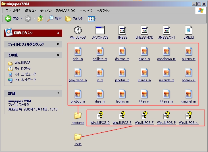
In the program version V7.2.03, the Help files are new.
Create one folder titled "_help" after unzipping
the program, and move the Help files. In V7.2.02,this step is necessary.
(In V7.2.01, this step is unnecessary.)
*Note* ---The first character in "_help" is an underscore.
The texture files in the directory "_textures" you need for texturing
planetary moons in Ehpemerides/Graphics.
 (V7.2.04)
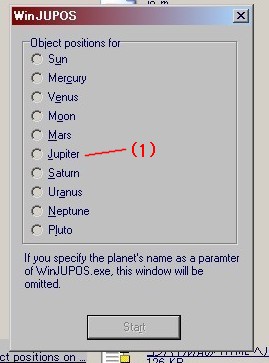
The selection window of the planets opens when the program is started for the first time.
Select "Jupiter (1)".
(V7.2.04)
The selection window of the planets opens when the program is started for the first time.
Select "Jupiter (1)".
 (V7.2.03)
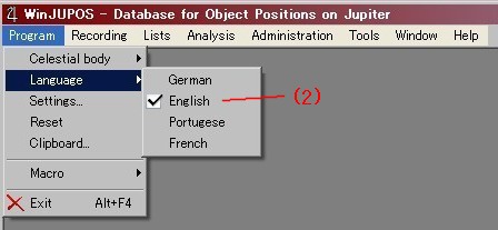
Click the icon of the program and the WinJUPOS screen opens.
Choose "English(2)" from"Language" in the drop down list. The default language is German.
*Note* ---The red sections in the English help file are not translated sections
from the German (original) version.
(V7.2.03)
Click the icon of the program and the WinJUPOS screen opens.
Choose "English(2)" from"Language" in the drop down list. The default language is German.
*Note* ---The red sections in the English help file are not translated sections
from the German (original) version.
 (V7.2.03)
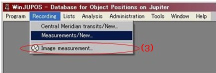
2 Importing images
2.1 Choose "Image measurement(3)" from the drop down list under "Recording".
(V7.2.03)
2 Importing images
2.1 Choose "Image measurement(3)" from the drop down list under "Recording".
 (V7.2.03)
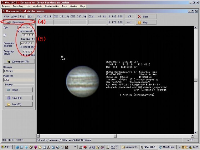
2.2 Click "Open image(4)". And the image is uploaded.
2.3 Input the observation date and time in UT.
Input the longitude of the observation site (East longitude is +)
and the latitude (North latitude is +). (5)
(V7.2.03)
2.2 Click "Open image(4)". And the image is uploaded.
2.3 Input the observation date and time in UT.
Input the longitude of the observation site (East longitude is +)
and the latitude (North latitude is +). (5)
 (V7.2.03)
---The date and time (UT) are used for CM calculation.
---Longitude and latitude are important for tropocentric co-ordinates and times for set and rise.
These values have no effect for C.M. latitudes of Jupiter.
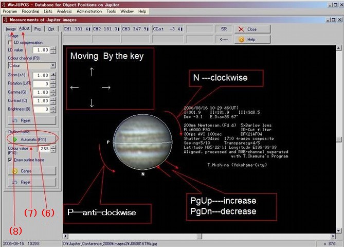
2.4 Click the "Adjust(6)" tab.
2.5 Click"Automatic(7)," and the outline and equator of Jupiter are displayed.
---Perform the keyboard operations (as written in the figure) when adjusting the position
of the circle by hand.
2.6 Choose the"Image(8)" tab, and save the image data.
The image data file is created in .ims format.
(V7.2.03)
---The date and time (UT) are used for CM calculation.
---Longitude and latitude are important for tropocentric co-ordinates and times for set and rise.
These values have no effect for C.M. latitudes of Jupiter.
2.4 Click the "Adjust(6)" tab.
2.5 Click"Automatic(7)," and the outline and equator of Jupiter are displayed.
---Perform the keyboard operations (as written in the figure) when adjusting the position
of the circle by hand.
2.6 Choose the"Image(8)" tab, and save the image data.
The image data file is created in .ims format.
 (V7.2.03)
Keyboard operation when the position of the circle is adjusted by hand
Arrow keys ---direction buttons for moving the outline
PgUp ---increases the size of the outline
PgDn ---decreases the size of the outline
N --- rotates the outline clockwise
P --- rotates the outline counterclockwise
Backspace --- rotates the outline by 180 degrees
Case of the south top image
Before 2.4 please choose the principle adjustment of the outline frame.
If south is top at your image rotate the outline frame in this way,
that "N" symbol is at bottom. Otherwise rotate "N" to top. Use the key
[Backspace] for this rotation (rotation of outline frame by 180 degrees).
*NOTE*---It is not the same result if you press
a) [F11] and then [Backspace] and
b) first [Backspace] and then [F11]
The background of this phenomenon is the limb darkening of the planets ellipse.
Case of the more than one planets images in one file
It is also possible to use the "Automatic adjustment" if you have more than one planetary images
in one file. In this case please decrease the Measurement window or zoom and move the image in
this way that you only see one full planetary body. After that press [F11].
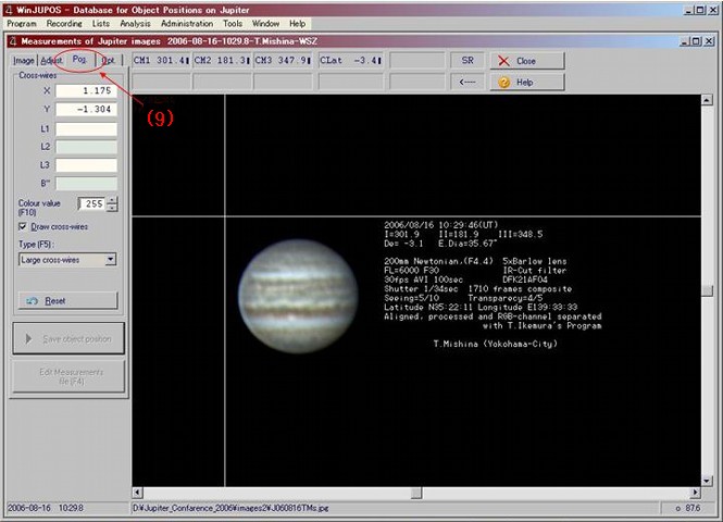
3 Positional measurement of planetary features
3.1 Select the "Pos.(9)" tab under "Measurement of (Jupiter) images."
(V7.2.03)
Keyboard operation when the position of the circle is adjusted by hand
Arrow keys ---direction buttons for moving the outline
PgUp ---increases the size of the outline
PgDn ---decreases the size of the outline
N --- rotates the outline clockwise
P --- rotates the outline counterclockwise
Backspace --- rotates the outline by 180 degrees
Case of the south top image
Before 2.4 please choose the principle adjustment of the outline frame.
If south is top at your image rotate the outline frame in this way,
that "N" symbol is at bottom. Otherwise rotate "N" to top. Use the key
[Backspace] for this rotation (rotation of outline frame by 180 degrees).
*NOTE*---It is not the same result if you press
a) [F11] and then [Backspace] and
b) first [Backspace] and then [F11]
The background of this phenomenon is the limb darkening of the planets ellipse.
Case of the more than one planets images in one file
It is also possible to use the "Automatic adjustment" if you have more than one planetary images
in one file. In this case please decrease the Measurement window or zoom and move the image in
this way that you only see one full planetary body. After that press [F11].
3 Positional measurement of planetary features
3.1 Select the "Pos.(9)" tab under "Measurement of (Jupiter) images."
 (V7.2.03)
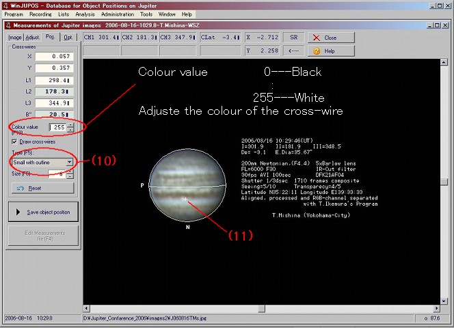
3.2 Choose the cross-wire type under "Type(10)".
There are four kinds cross-wire and outline types
(large cross-wire, small cross-wire, large cross-wire with an outline,
small cross-wire with an outline).
3.3 You can measure the position by matching up the cross-wire directly with the planetary feature.(11)
(V7.2.03)
3.2 Choose the cross-wire type under "Type(10)".
There are four kinds cross-wire and outline types
(large cross-wire, small cross-wire, large cross-wire with an outline,
small cross-wire with an outline).
3.3 You can measure the position by matching up the cross-wire directly with the planetary feature.(11)
 (V7.2.03)
4 Making drift charts
4.1 Preparation
4.1.1 Decide the method for arranging the record of the measurement data.
---Method of creating measurement data files for each observer.
It is highly recommended to use only "Method of creating measurement
data files for each observer.Every observer gets one Measurement file (*.mea)
4.1.2 Creating a project folder
---Create a folder that contains the measurement data.
Two or more measurement data files are placed in the same folder.
---Create a folder at the output destination for the drift chart.
(V7.2.03)
4 Making drift charts
4.1 Preparation
4.1.1 Decide the method for arranging the record of the measurement data.
---Method of creating measurement data files for each observer.
It is highly recommended to use only "Method of creating measurement
data files for each observer.Every observer gets one Measurement file (*.mea)
4.1.2 Creating a project folder
---Create a folder that contains the measurement data.
Two or more measurement data files are placed in the same folder.
---Create a folder at the output destination for the drift chart.
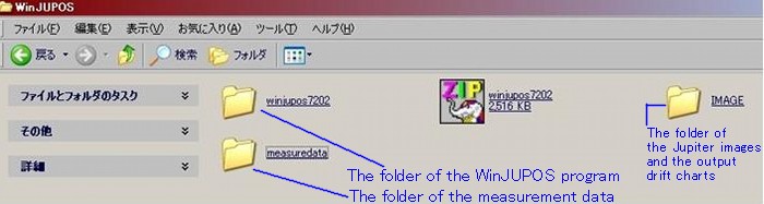
Hahn's directory structure is:
D:\WinJUPOS
\_help
\_textures
\Jupiter
\Images
\2005 (date-observer name-info.jpg)
\2006 (date-observer name-info.jpg)
\Measurements (observer name.mea)
\Central Meridian timings (observer name.cmt)
\Selections (object name-info.wse)
\_Settings
\Image Measurements (*.ims)
\Selections (*.ses)
\Drift charts (*.grs)
\Map computations (*.mcs)
\Image computations (*.ics)
\Drift charts (*.gif)
\Maps (*.jpg)
\Saturn
...
\Uranus
...
|
*NOTE* --- For international data exchanging I highly recommend to use only pure ASCII
characters (= English) for directory and file names, observer names and addresses,
image info. But you do not need it, if you use the data only in your own country.
4.2 Creating and initialization of measurement data files
4.2.1 Start WinJUPOS.
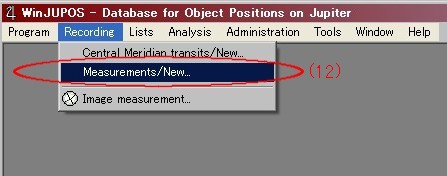
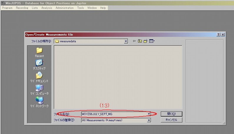
4.2.2 Select "Measurements/New(12)" from the drop down list under "Recording." Enter the file name.(13)
 (V7.2.03)
 (V7.2.03)
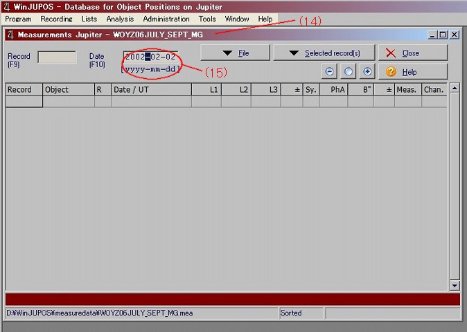
4.2.3 A new file is opened, and initial screen(14) is displayed.
4.2.4 Input the "Date(15)".
(V7.2.03)
4.2.3 A new file is opened, and initial screen(14) is displayed.
4.2.4 Input the "Date(15)".
 (V7.2.03)
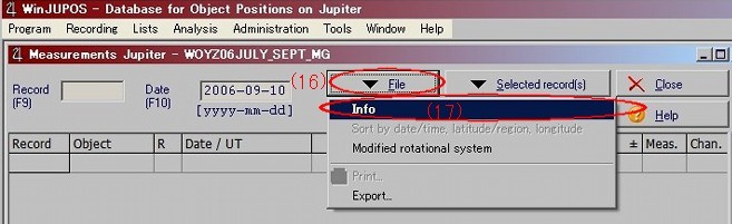
4.2.5 Click the "File button(16)", and select "Info(17)" from the drop down list.
(V7.2.03)
4.2.5 Click the "File button(16)", and select "Info(17)" from the drop down list.
 (V7.2.03)
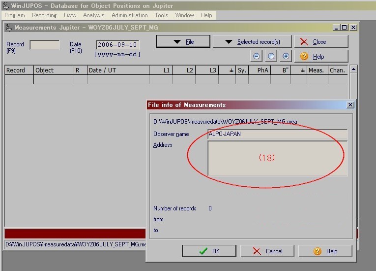
4.2.6 Type the "Observer name" and"Address".(18)
---You will type the latitude and longitude of the address, e-mail address,
and the observation location.
---You can edit these data at every time if you open the Measurement file
via "Recording - Measurements/New..."
(V7.2.03)
4.2.6 Type the "Observer name" and"Address".(18)
---You will type the latitude and longitude of the address, e-mail address,
and the observation location.
---You can edit these data at every time if you open the Measurement file
via "Recording - Measurements/New..."
 (V7.2.03)
Exsample
Toshihiko Ikemura gets the file "Ikemura.mea"
The "Observer name" is "Ikemura, Toshihiko"
The "Address" is "Nagoya City, J"
All observations / object positions of Toshihiko Ikemura will be stored in "Ikemura.mea".
4.3 Recording of measurement data
4.3.1 Select "Image measurement" in the drop down list under "Recording".
(The image processed immediately before is displayed. )
4.3.2 Follow the steps in "2 Importing images" and "3 Positional measurement of planetary features"
when you measure a new image.
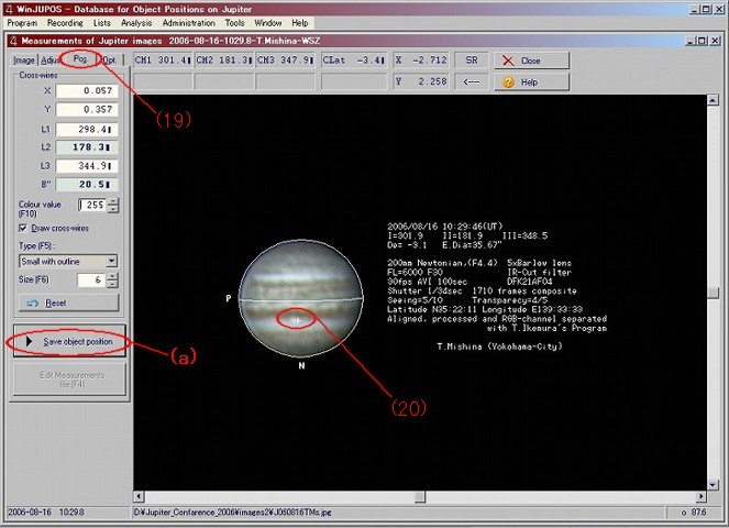
4.3.3 Select the "Pos.(19)" tab, the measurement screen is displayed.
4.3.4 Match the cross-wire(20) on planetary feature and click. Click "Save object position button (a) ".
(V7.2.03)
Exsample
Toshihiko Ikemura gets the file "Ikemura.mea"
The "Observer name" is "Ikemura, Toshihiko"
The "Address" is "Nagoya City, J"
All observations / object positions of Toshihiko Ikemura will be stored in "Ikemura.mea".
4.3 Recording of measurement data
4.3.1 Select "Image measurement" in the drop down list under "Recording".
(The image processed immediately before is displayed. )
4.3.2 Follow the steps in "2 Importing images" and "3 Positional measurement of planetary features"
when you measure a new image.
4.3.3 Select the "Pos.(19)" tab, the measurement screen is displayed.
4.3.4 Match the cross-wire(20) on planetary feature and click. Click "Save object position button (a) ".
 (V7.2.03)
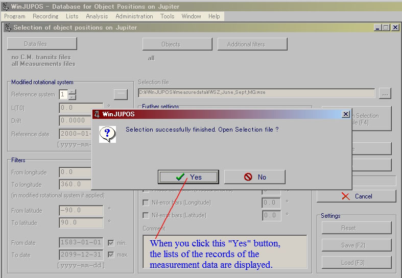
4.3.5 The window (b) of the data input appears.
Input the observation pattern type in the column for"Code (c)."
(See the explanation in the following section 4.3.7.)
(A question mark sign "_" is displayed in the column for"Code." This"_" is a delimiter.)
4.3.6 Click the "Save (d) " button. Then, the record of the measurement data is added.
(V7.2.03)
4.3.5 The window (b) of the data input appears.
Input the observation pattern type in the column for"Code (c)."
(See the explanation in the following section 4.3.7.)
(A question mark sign "_" is displayed in the column for"Code." This"_" is a delimiter.)
4.3.6 Click the "Save (d) " button. Then, the record of the measurement data is added.
vve.jpg) (V7.2.04)
4.3.7 Concerning the input for the"Code" column
---Ahead of the question mark sign "_"
1st letter : W-- for a bright object,
D-- for a dark object,
2nd letter : P-- preceding side,
C-- centre,
F-- following side,
3rd letter : 1-- if the object was easy,
2-- if the object was moderate,
3-- if the object was difficult to see (in case this information is available)
---After the question mark sign "_"
Bright object : SPTR, ASPOT, OVAL, BAY, NICK, GAP, SECT, RIFT, AREA, STRK
Dark object : SDER, SPOT, BAR, FEST, PROJ, SECT, VEIL, DIST,COL, STRK
Look at the Object code Jupiter (JUPOS) in the Image measurement Help section,
if you want to know in detail.
*NOTE*--- Your "Measurer code" you get from Hans-Joerg Mettig/Germany, if you want to measure
object positions for the international WinJUPOS database.
4.4 Making drift charts
4.4.1 Step1 Data compilation
4.4.1.1 Choose the "Selection (e)" from the drop down list under "Analysis".
(V7.2.04)
4.3.7 Concerning the input for the"Code" column
---Ahead of the question mark sign "_"
1st letter : W-- for a bright object,
D-- for a dark object,
2nd letter : P-- preceding side,
C-- centre,
F-- following side,
3rd letter : 1-- if the object was easy,
2-- if the object was moderate,
3-- if the object was difficult to see (in case this information is available)
---After the question mark sign "_"
Bright object : SPTR, ASPOT, OVAL, BAY, NICK, GAP, SECT, RIFT, AREA, STRK
Dark object : SDER, SPOT, BAR, FEST, PROJ, SECT, VEIL, DIST,COL, STRK
Look at the Object code Jupiter (JUPOS) in the Image measurement Help section,
if you want to know in detail.
*NOTE*--- Your "Measurer code" you get from Hans-Joerg Mettig/Germany, if you want to measure
object positions for the international WinJUPOS database.
4.4 Making drift charts
4.4.1 Step1 Data compilation
4.4.1.1 Choose the "Selection (e)" from the drop down list under "Analysis".
v.jpg) (V7.2.03)
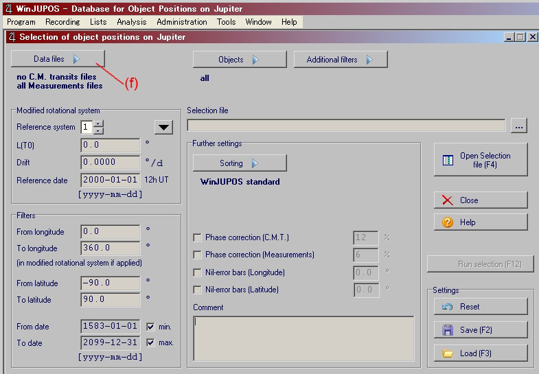
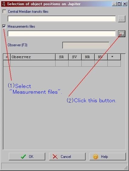
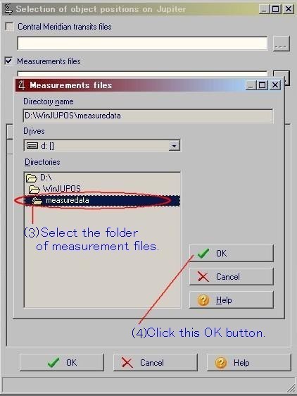
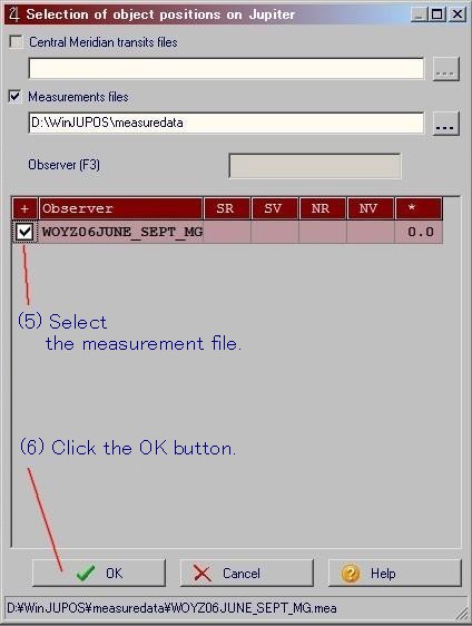
4.4.1.2 Select the file that contains the record of the measurement data from"Data file (f)."
(Place two or more data files in the folder. When each folder is selected,
the data file list is displayed.Select the data file to be used for making the drift chart.)
(V7.2.03)
4.4.1.2 Select the file that contains the record of the measurement data from"Data file (f)."
(Place two or more data files in the folder. When each folder is selected,
the data file list is displayed.Select the data file to be used for making the drift chart.)
 (V7.2.04)
 (V7.2.03)
 (V7.2.03)
 (V7.2.03)
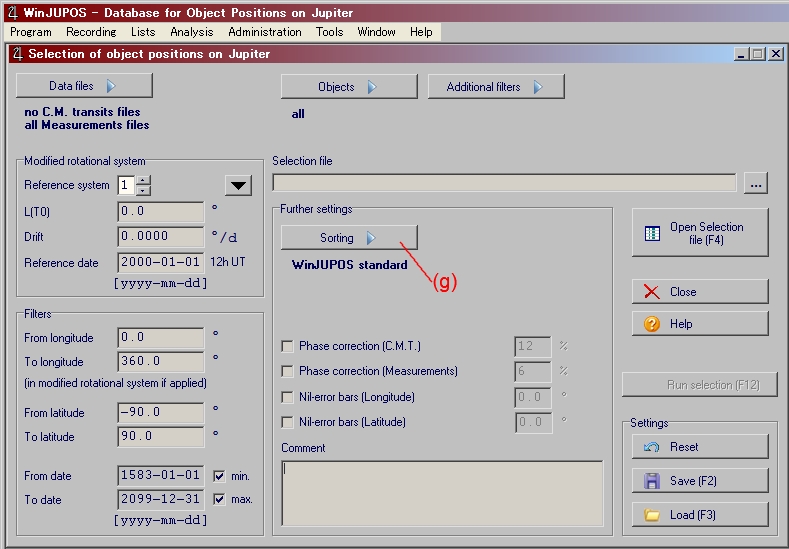
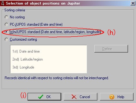
4.4.1.3 Click the Sorting button (g).
(V7.2.03)
4.4.1.3 Click the Sorting button (g).
 (V7.2.04)
Click"WinJUPOS Standard... (h)" and click the "OK button (i)", and the data is sorted.
(V7.2.04)
Click"WinJUPOS Standard... (h)" and click the "OK button (i)", and the data is sorted.
 (V7.2.03)
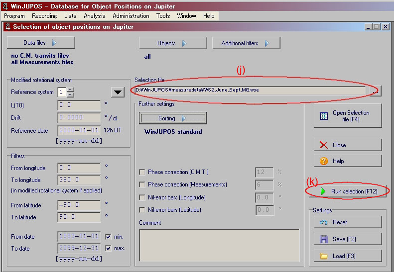
4.4.1.4 Set the output file with Selection file (j).
(It is a good idea to include the date in the file name.)
4.4.1.5 Click "Run selection (k)". Processing is executed.
(V7.2.03)
4.4.1.4 Set the output file with Selection file (j).
(It is a good idea to include the date in the file name.)
4.4.1.5 Click "Run selection (k)". Processing is executed.
 (V7.2.04)
 (V7.2.04)
4.4.2 Step2 Drawing a drift chart
4.4.2.1 Choose "Drift Chart (l)" from the drop down list under "Analysis".
(V7.2.04)
4.4.2 Step2 Drawing a drift chart
4.4.2.1 Choose "Drift Chart (l)" from the drop down list under "Analysis".
vv.jpg) (V7.2.03)
4.4.2.2 The window for the file specification appears when you click the "Data file button (m) ".
Specify the file set by the section 4.4.1.4 in 4.4.1 step 1.
(When you select the folder, the list of the data file is displayed.)
(V7.2.03)
4.4.2.2 The window for the file specification appears when you click the "Data file button (m) ".
Specify the file set by the section 4.4.1.4 in 4.4.1 step 1.
(When you select the folder, the list of the data file is displayed.)
vv.jpg) (V7.2.04)
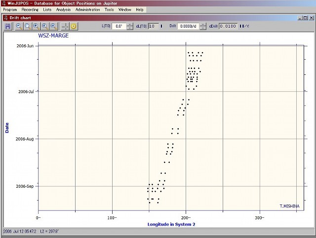
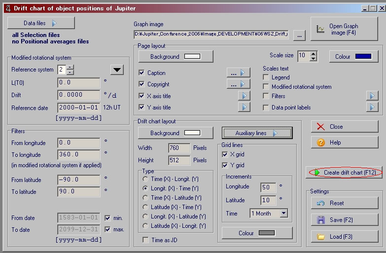
4.4.2.3 Enter the output file name in the "Graph image column(n)."
4.4.2.4 "Longit.(x) - Time(y)" is good for "Type (o)".
4.4.2.5 Click "Create drift chart (p)". Processing is executed.
(V7.2.04)
4.4.2.3 Enter the output file name in the "Graph image column(n)."
4.4.2.4 "Longit.(x) - Time(y)" is good for "Type (o)".
4.4.2.5 Click "Create drift chart (p)". Processing is executed.
VVE.jpg) (V7.2.04)
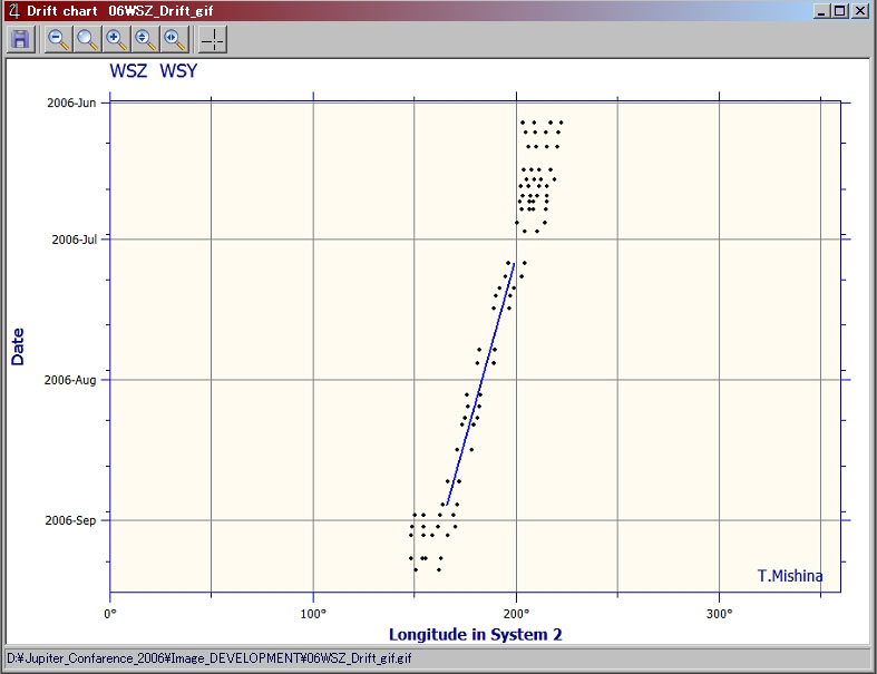
Example of the drift chart
(V7.2.04)
Example of the drift chart
 (V7.2.03)
4.4.3 STEP3 Auxiliary lines
4.4.3.1 Using the drift data for "Auxiliary lines" in Drift charts.
4.4.3.2 Drift computation
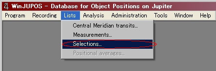
4.4.3.2.1 Choose the "Selections" from the drop down list under "Lists".
(V7.2.03)
4.4.3 STEP3 Auxiliary lines
4.4.3.1 Using the drift data for "Auxiliary lines" in Drift charts.
4.4.3.2 Drift computation
4.4.3.2.1 Choose the "Selections" from the drop down list under "Lists".
 (V7.2.04)
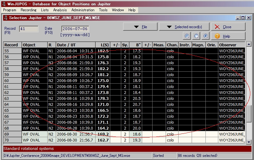
4.4.3.2.2 Select all records of one object for Drift computation
(V7.2.04)
4.4.3.2.2 Select all records of one object for Drift computation
 (V7.2.04)
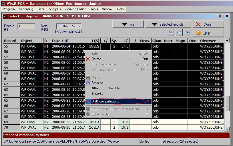
4.4.3.2.3 Press right mouse button and call "Drift computation"
(V7.2.04)
4.4.3.2.3 Press right mouse button and call "Drift computation"
 (V7.2.04)
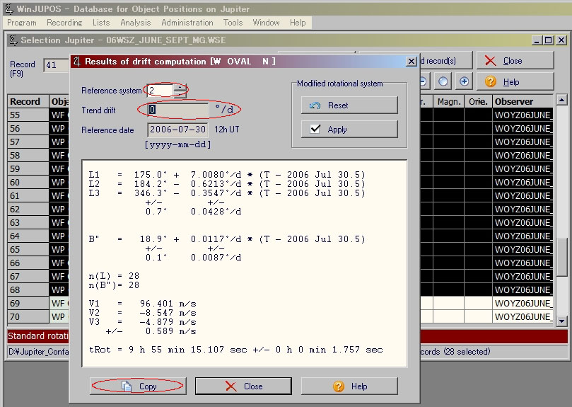
4.4.3.2.4 Choose the "Reference system" and the "Trend drift" and
press "Copy" if drift computation is correct.
(V7.2.04)
4.4.3.2.4 Choose the "Reference system" and the "Trend drift" and
press "Copy" if drift computation is correct.
 (V7.2.04)
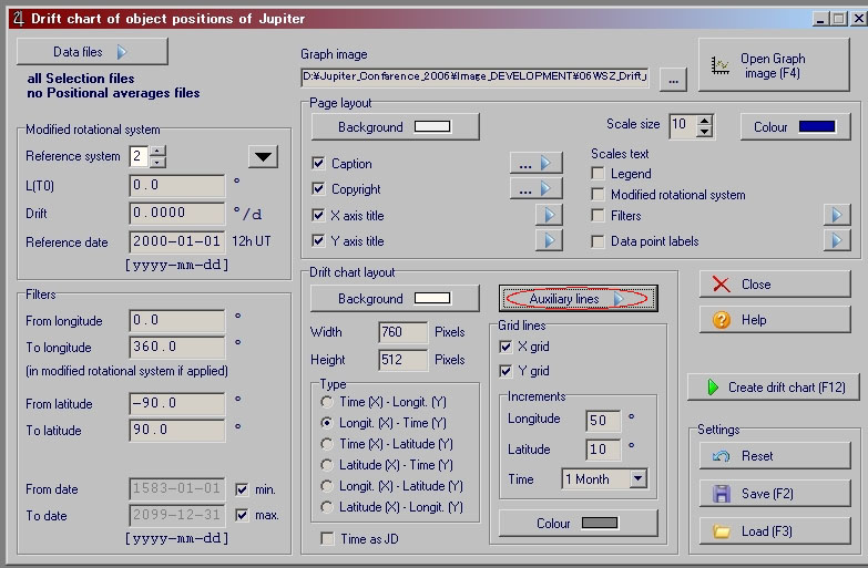
4.4.3.3 Drawing a drift chart with the auxiliary lines
4.4.3.3.1 Choose "Drift Chart" from the drop down list under "Analysis".
4.4.3.3.2 Click "Auxiliary lines"
(V7.2.04)
4.4.3.3 Drawing a drift chart with the auxiliary lines
4.4.3.3.1 Choose "Drift Chart" from the drop down list under "Analysis".
4.4.3.3.2 Click "Auxiliary lines"
 (V7.2.04)
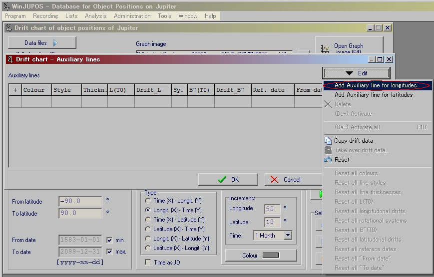
4.4.3.3.3 Choose "Add auxiliary line for longitude" from the drop down list under "Edit".
(V7.2.04)
4.4.3.3.3 Choose "Add auxiliary line for longitude" from the drop down list under "Edit".
 (V7.2.04)
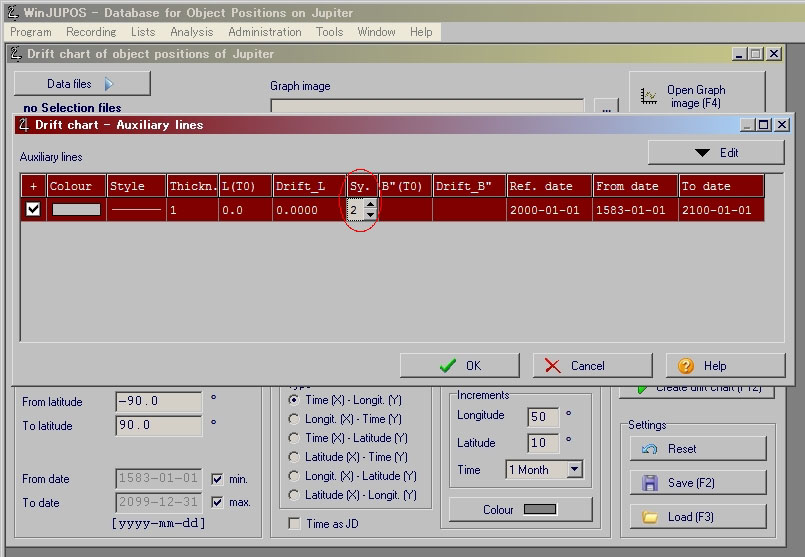
4.4.3.3.4 Select rotational system "Sy."
(V7.2.04)
4.4.3.3.4 Select rotational system "Sy."
 (V7.2.04)
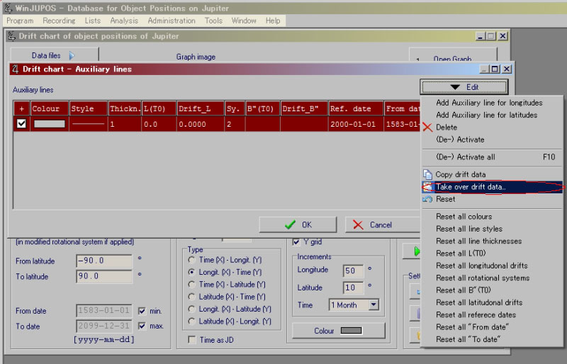
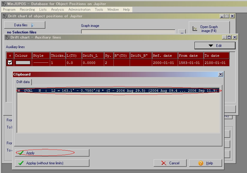
4.4.3.3.5 Choose "Take over drift data" from the drop down list under "Edit".
(V7.2.04)
4.4.3.3.5 Choose "Take over drift data" from the drop down list under "Edit".
 (V7.2.04)
4.4.3.3.6 Select drift record and Click "Apply"
(V7.2.04)
4.4.3.3.6 Select drift record and Click "Apply"
 (V7.2.04)
4.4.3.3.7 Click "Ok" button.
4.4.3.3.8 Click "Create drifft chart" button,compute a drift chart in the same rotational system
(V7.2.04)
4.4.3.3.7 Click "Ok" button.
4.4.3.3.8 Click "Create drifft chart" button,compute a drift chart in the same rotational system
 (V7.2.04)
Exsample the drift chart with the auxiliary line
(V7.2.04)
Exsample the drift chart with the auxiliary line
 (V7.2.04)
The file formats are BMP, Jpeg,amd Gif etc.
You can write the explanation sentence by using the retouching software or the paint software
(MS paint and PictBear).
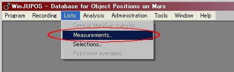
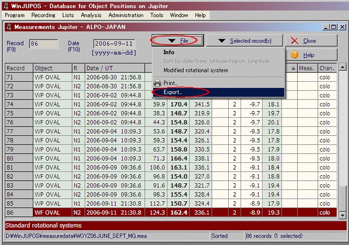
4.5 Export (to CSV) of measurement data of the planets
4.5.1 Choose "Measurement" from the drop down list under "Lists".
(V7.2.04)
The file formats are BMP, Jpeg,amd Gif etc.
You can write the explanation sentence by using the retouching software or the paint software
(MS paint and PictBear).
4.5 Export (to CSV) of measurement data of the planets
4.5.1 Choose "Measurement" from the drop down list under "Lists".
 (V7.2.03)
4.5.2 Click"File", and the drop down list is displayed. Choose "Export" from this drop down list.
(V7.2.03)
4.5.2 Click"File", and the drop down list is displayed. Choose "Export" from this drop down list.
 (V7.2.03)
5 Making projection maps
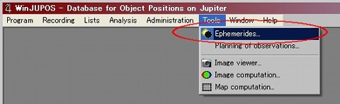
5.1 Choose "Map computation" from the drop down list under "Tools".
5.2 Click"Edit (q)", and the drop down list is displayed.
Click"Add (r)" to upload picture files (.ims format) that have been saved.
(V7.2.03)
5 Making projection maps
5.1 Choose "Map computation" from the drop down list under "Tools".
5.2 Click"Edit (q)", and the drop down list is displayed.
Click"Add (r)" to upload picture files (.ims format) that have been saved.
vv.jpg) (V7.2.03)
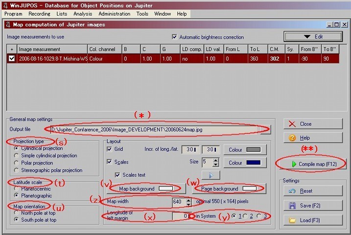
5.3 Choose the "Projection type (s)." The default is"Cylindrical projection".
The"Latitude scale (t)" seems best to be left at the default setting (Planetographic).
5.4 Choose the"Map orientation(u) ". (North pole at top /South pole at top)
5.5 Choose the color of "Grid", "Scales"," Map background (v) " and "Page background (w) ".
5.6 Set "Longitude of left margin(x)" and "SYSTEM, 1, 2, and 3(y)".
5.7 Set a "Map Width (z)" of an appropriate size.
5.8 Specify the "Output file(*)"
5.9 Execute "Compile map(**)".
5.10 Adjust the "Longitude of left margin" set in the section 5.6 when the position of the planet shifts.
(V7.2.03)
5.3 Choose the "Projection type (s)." The default is"Cylindrical projection".
The"Latitude scale (t)" seems best to be left at the default setting (Planetographic).
5.4 Choose the"Map orientation(u) ". (North pole at top /South pole at top)
5.5 Choose the color of "Grid", "Scales"," Map background (v) " and "Page background (w) ".
5.6 Set "Longitude of left margin(x)" and "SYSTEM, 1, 2, and 3(y)".
5.7 Set a "Map Width (z)" of an appropriate size.
5.8 Specify the "Output file(*)"
5.9 Execute "Compile map(**)".
5.10 Adjust the "Longitude of left margin" set in the section 5.6 when the position of the planet shifts.
 (V7.2.03)
6 Ephemeris and positional display of satellites
6.1 Preparation
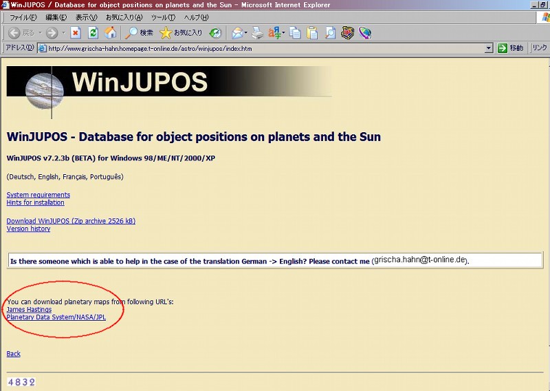
The texture maps for the planets can be downloaded from the NASA website or the website
of James Hastings beforehand. (These are linked from Grischa Hahn's website. )
For the texture maps from NASA, the longitude on the edge is 180 degrees.
For the texture maps from James Hasting's website, the longitude on the edge is 0 degrees.
(V7.2.03)
6 Ephemeris and positional display of satellites
6.1 Preparation
The texture maps for the planets can be downloaded from the NASA website or the website
of James Hastings beforehand. (These are linked from Grischa Hahn's website. )
For the texture maps from NASA, the longitude on the edge is 180 degrees.
For the texture maps from James Hasting's website, the longitude on the edge is 0 degrees.
 6.2 Displaying the Ephemeris window
6.2.1 Choose "Ephemerides" under "Toole".
6.2 Displaying the Ephemeris window
6.2.1 Choose "Ephemerides" under "Toole".
 (V7.2.03)
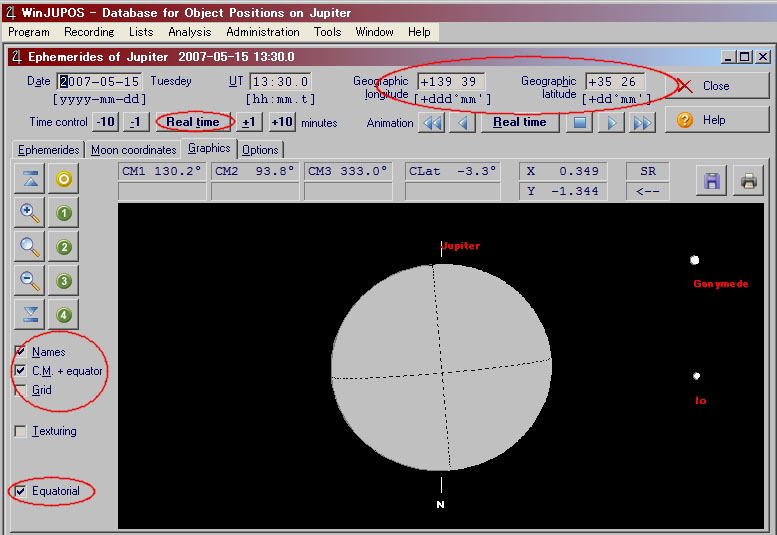
6.2.2 Choose the "Graphics tab".
Enter the latitude and the longitude of the observation site.
When the "Real time button" is clicked, the current date and time in UT are displayed.
"Names" (of the satellites),"C.M.+equator" and "Equatorial" can be selected under the "Graphics" tab.
(V7.2.03)
6.2.2 Choose the "Graphics tab".
Enter the latitude and the longitude of the observation site.
When the "Real time button" is clicked, the current date and time in UT are displayed.
"Names" (of the satellites),"C.M.+equator" and "Equatorial" can be selected under the "Graphics" tab.
 (V7.2.04)
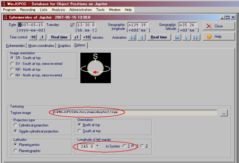
6.2.3 Choose the "Options tab".
Specify the texture map of the planets that was downloaded in Preparation step 6.1,
under "Texture image."
Adjust the "Longitude of left margin" to 180 for the texture maps from NASA.
Adjust the "Longitude of left margin" to 245 for the texture map of Cassini's image
on James Hastings' web site, then GRS is on longitude 115.
t(For the texture maps, they can also be made from creating projection charts
using your own planetary images, and then doing a montage.)
(V7.2.04)
6.2.3 Choose the "Options tab".
Specify the texture map of the planets that was downloaded in Preparation step 6.1,
under "Texture image."
Adjust the "Longitude of left margin" to 180 for the texture maps from NASA.
Adjust the "Longitude of left margin" to 245 for the texture map of Cassini's image
on James Hastings' web site, then GRS is on longitude 115.
t(For the texture maps, they can also be made from creating projection charts
using your own planetary images, and then doing a montage.)
 (V7.2.04)
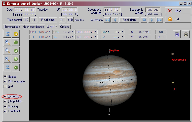
6.2.4 Choose the "Graphics tab".
When "Texturing" is specified, the image is displayed.
(V7.2.04)
6.2.4 Choose the "Graphics tab".
When "Texturing" is specified, the image is displayed.
 (V7.2.04)
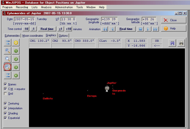
A wide-field view is displayed when the "minus" button is clicked,
and you can identify the location of the satellites.
(V7.2.04)
A wide-field view is displayed when the "minus" button is clicked,
and you can identify the location of the satellites.
 (V7.2.04)
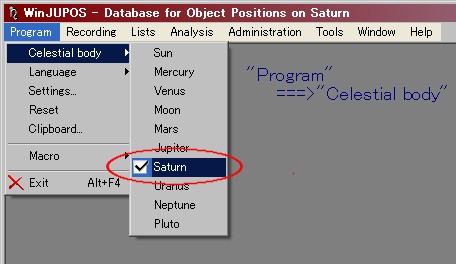
7 Mars, Saturn, and the Sun, etc.
The object is specified under the drop down list by clicking the "Program tab"
when the program starts.
(V7.2.04)
7 Mars, Saturn, and the Sun, etc.
The object is specified under the drop down list by clicking the "Program tab"
when the program starts.
 (V7.2.03)
7.1 Choose "Image measurement" from the drop down list under"Recording".
7.2 Import images by clicking "Open image".
7.3 Input the observation date and time in UT.
Input the longitude of the observation site (East longitude is +)
and the latitude (North latitude is +).
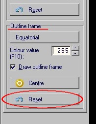
7.4 Select the"Adjust tab".
7.5 Click"Draw outline frame".(Click the "Reset" button if the outline is not displayed.)
(V7.2.03)
7.1 Choose "Image measurement" from the drop down list under"Recording".
7.2 Import images by clicking "Open image".
7.3 Input the observation date and time in UT.
Input the longitude of the observation site (East longitude is +)
and the latitude (North latitude is +).
7.4 Select the"Adjust tab".
7.5 Click"Draw outline frame".(Click the "Reset" button if the outline is not displayed.)
 (V7.2.03)
Keyboard operation when the position of the circle is adjusted by hand.
arrow keys --- moves the outline
PgUp --- increases the size of the outline
PgDn --- decreases the size of the outline
N --- rotates the outline clockwise
P --- rotates the outline counterclockwise
Backspace --- rotates the outline by 180 degrees
7.6 Choose the "Image tab", and save the image data.
---The measurement of the position is performed the same way as with Jupiter.
---The projection maps are created the same way as with Jupiter.
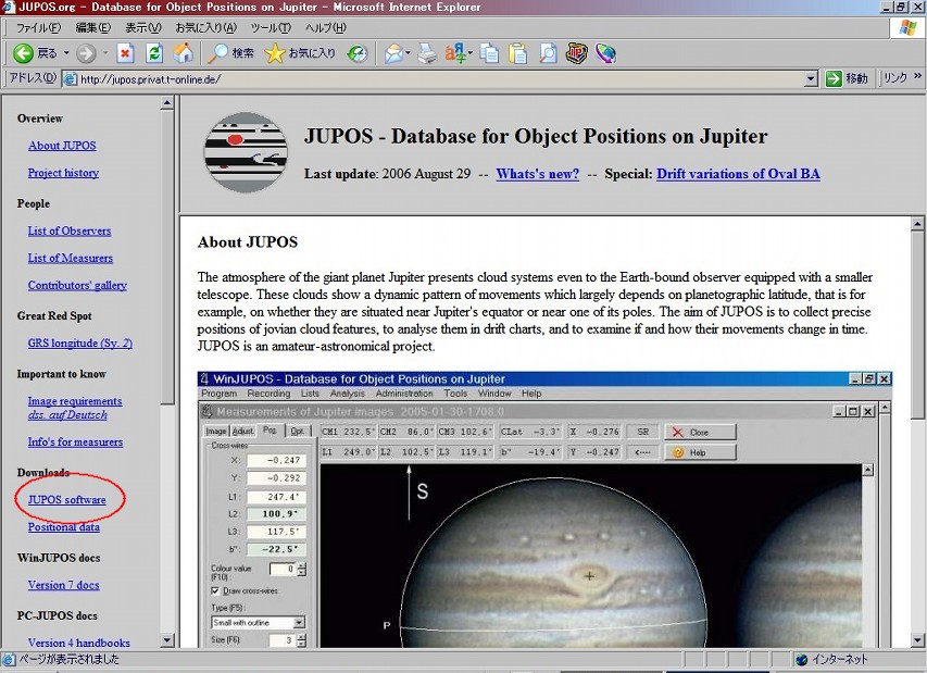
8 Download web site
WinJUPOS can be downloaded from the site ( http://jupos.privat.t-online.de/ ) of JUPOS.
Download "WinJUPOS v7.x.x Multi-planet, multi-lingual".
(V7.2.03)
Keyboard operation when the position of the circle is adjusted by hand.
arrow keys --- moves the outline
PgUp --- increases the size of the outline
PgDn --- decreases the size of the outline
N --- rotates the outline clockwise
P --- rotates the outline counterclockwise
Backspace --- rotates the outline by 180 degrees
7.6 Choose the "Image tab", and save the image data.
---The measurement of the position is performed the same way as with Jupiter.
---The projection maps are created the same way as with Jupiter.
8 Download web site
WinJUPOS can be downloaded from the site ( http://jupos.privat.t-online.de/ ) of JUPOS.
Download "WinJUPOS v7.x.x Multi-planet, multi-lingual".
 Acknowledgements
I would like to express my gratitude to Mr. Robert Heffner who corrected my English draft.
END
Acknowledgements
I would like to express my gratitude to Mr. Robert Heffner who corrected my English draft.
END